Methods and Evaluation Protocol for the Progress-State Regime Gate
This note documents the evaluation workflow used for the progress-state “regime gate” experiments on crypto candles. The emphasis is methodological: definition of the gate, the mapping from price history to a bounded setting, the backtest and walk-forward protocol, friction modelling, and how parameter pockets are selected and recorded.
The gate is treated as a controller layer that can sit on top of other signals. It is not presented as a complete trading system or an “alpha” in isolation.
1. Model definition
The gate maintains a small internal state per run:
σ ∈ {+1, -1} (orientation / regime sign), and p ∈ [0, 1) (progress accumulator).
Each bar supplies a scalar “setting” (an angle-like value). An alignment test compares the setting to a reference parameter λ and selects a two-level push δ:
- δ = δhi when the setting is within a window width w of λ (an “aligned” state)
- δ = δlo otherwise (a “weak” state)
The accumulator advances p ← p + δ. Let n = ⌊p⌋, and reset p ← p - n (so p ∈ [0, 1) again). Orientation flips when n is odd (parity of crossings). This makes the update arithmetic-only (adds, floor, comparisons, sign flip).
2. Feature to setting mapping
Price history is mapped to a bounded “setting” in [-π, π]. The current implementation uses a momentum-style feature over a lookback L:
- Compute momentum over L bars (e.g. percent change)
- Normalize by a robust scale (standard deviation with ε guard)
- Squash with arctan to obtain a bounded angle-like setting
This mapping is intentionally simple. The gate is a controller; different features can be substituted without changing the gate mechanics.
3. Trading policy
The policy converts σ into a target position. Two common profiles are supported:
- Long-only: σ = +1 → long; σ = -1 → flat
- Long/short: σ = +1 → long; σ = -1 → short (with a configurable short_scale, often 0.5 or 1.0)
A minimum holding period (min_hold) is enforced to reduce turnover. For intraday data, this is treated as a minimum number of bars.
4. Friction model (fees / slippage bucket)
Execution friction is modelled as a per-turn cost in basis points (bps) whenever the position changes. The core stress buckets are:
- 10 bps (optimistic / good execution)
- 25 bps (moderate / realistic for careful execution)
- 50 bps (pessimistic / “hard mode”)
The objective is not to perfectly model microstructure. The objective is to test whether parameter pockets remain viable under materially different friction assumptions.
5. In-sample backtest (debugging / intuition)
A full-history backtest is run for rapid iteration and debugging. This produces an equity curve, a σ time series, and a timeseries output suitable for inspection. In-sample results are not used as the primary evidence for robustness.
6. Walk-forward evaluation
The main evaluation protocol is walk-forward testing using rolling train/test windows aligned to calendar years. For each window:
- Define training span (e.g. 4 years) and test span (e.g. 1 year)
- Evaluate the gate on the test window only (out-of-sample)
- Stitch test windows to form a continuous OOS equity series
Outputs include: per-window summary metrics, a stitched OOS series, an OOS equity plot, and a meta JSON that records the configuration and results for auditability.
7. Metrics reported
- Annualized return and annualized volatility (using a bars-per-year constant)
- Sharpe = μ / σ (no claims about stationarity; used as a coarse comparator)
- Max drawdown on the stitched OOS equity series
- Turns (number of position changes) as a proxy for turnover and friction sensitivity
8. Parameter search and “pocket” selection
Parameter tuning is treated as a search for stable pockets, not a search for a single perfect configuration. Typical tuned parameters include:
- setting lookback L
- alignment window w
- δ_hi and δ_lo
- min_hold
- short_scale
Two scoring styles are supported:
- Mean score across assets/fees (captures average behaviour)
- Worst-window penalty (discourages configurations that fail badly in any single window)
Timeframes are treated separately. Daily, 6h, and 1h data produce different viable pockets, and the search ranges are adjusted accordingly.
9. Results snapshot
This section records a current results snapshot using the walk-forward stitched out-of-sample protocol and friction buckets (10/25/50 bps). These are empirical pockets rather than fixed claims; results can drift as timeframes, features, or market regimes change.
1d (daily) canon — stitched OOS
Canon: lb=180, w=0.30, δ_hi/δ_lo=0.85/0.20, hold=30, short_scale=1.0. Fees: 10 / 25 / 50 bps.
BTC
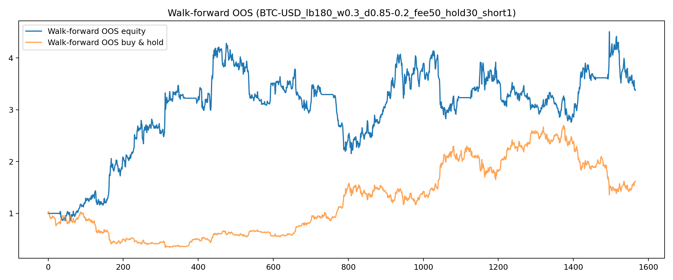
- fee10: ann_return 0.3263, Sharpe 0.6562, maxDD -0.4764
- fee25: ann_return 0.3103, Sharpe 0.6237, maxDD -0.4842
- fee50: ann_return 0.2835, Sharpe 0.5695, maxDD -0.4970
ETH
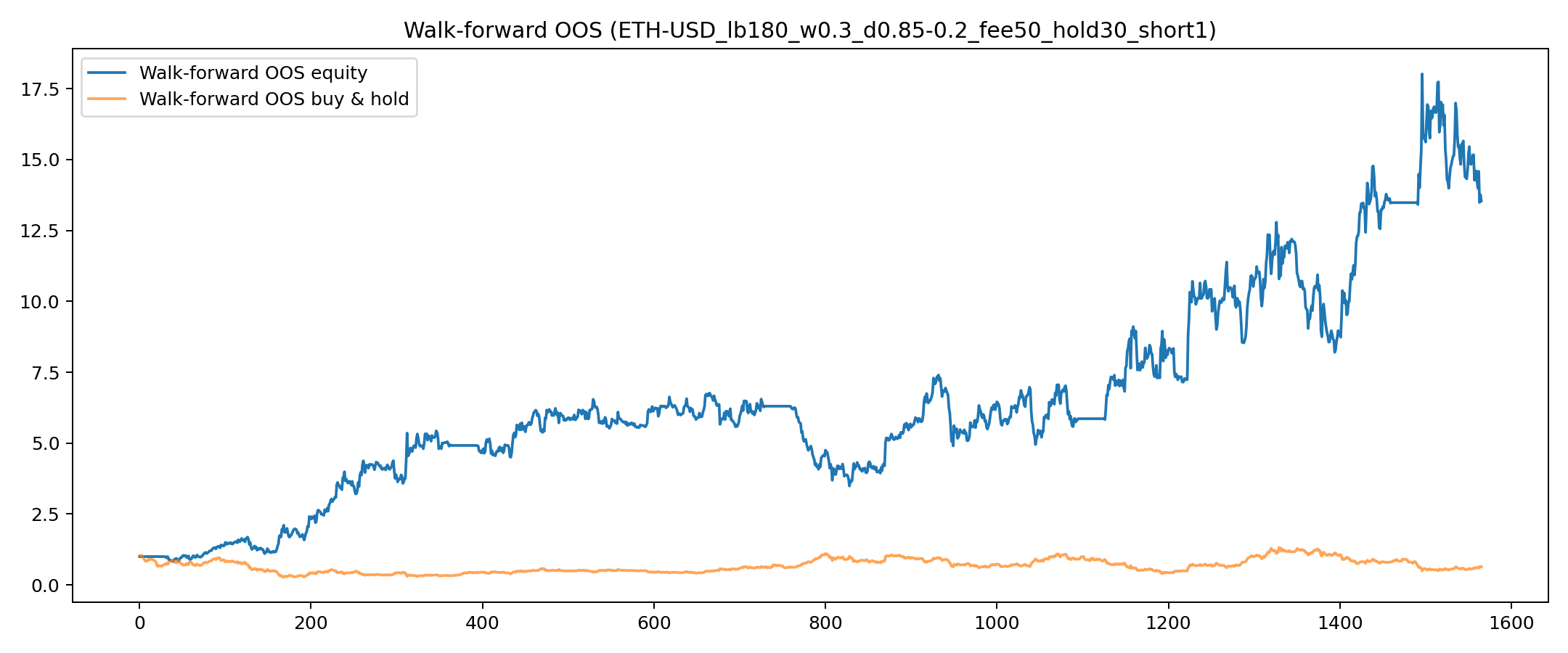
- fee10: ann_return 0.6503, Sharpe 0.9690, maxDD -0.4735
- fee25: ann_return 0.6342, Sharpe 0.9449, maxDD -0.4774
- fee50: ann_return 0.6074, Sharpe 0.9047, maxDD -0.4839
Takeaway: smooth degradation with fees on this pocket; ETH is stronger than BTC on this particular daily canon.
6h canon — stitched OOS
Canon: lb=360, w=0.30, δ_hi/δ_lo=0.90/0.15, hold=30 bars, short_scale=0.5. Fees: 10 / 25 / 50 bps.
ETH (short0.5)
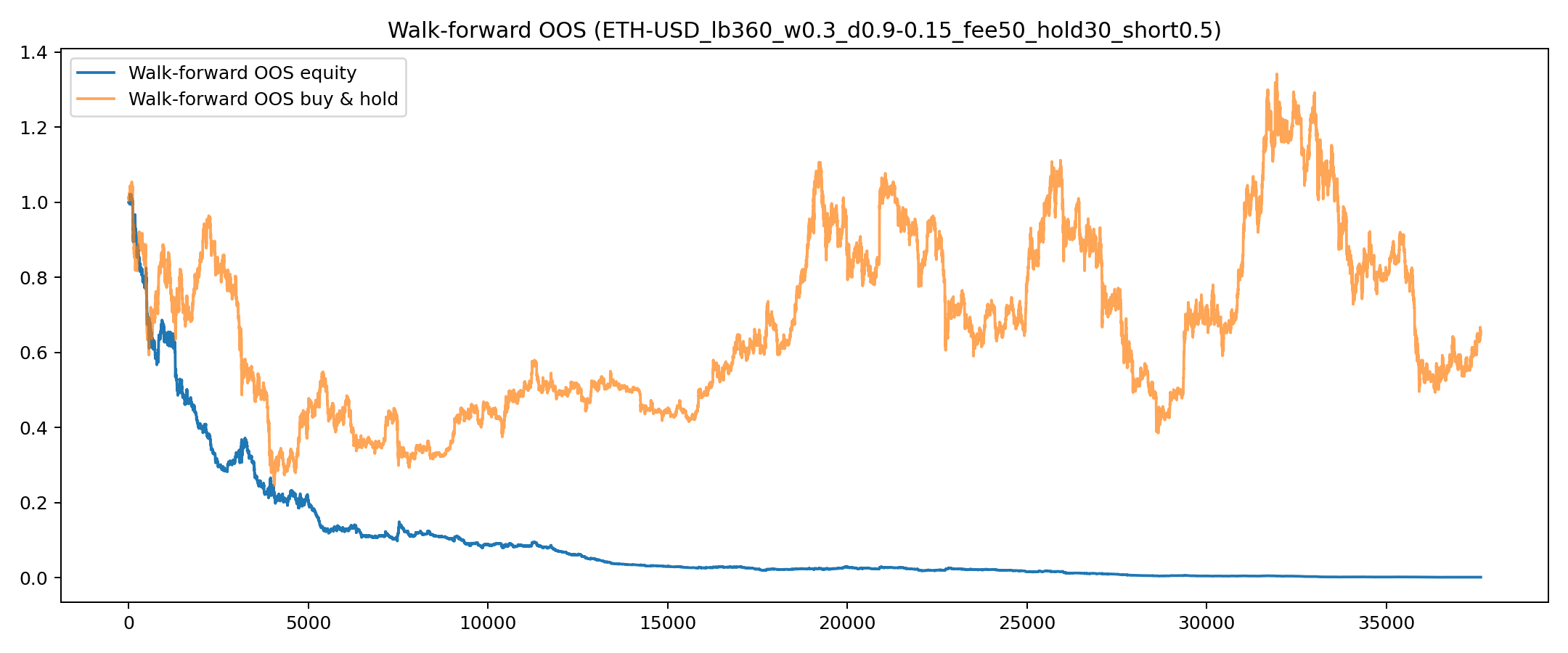
- fee10: ann_return 0.6126, Sharpe 1.0112, maxDD -0.5581
- fee25: ann_return 0.5466, Sharpe 0.9021, maxDD -0.5705
- fee50: ann_return 0.4365, Sharpe 0.7200, maxDD -0.5904
BTC (short0.5)
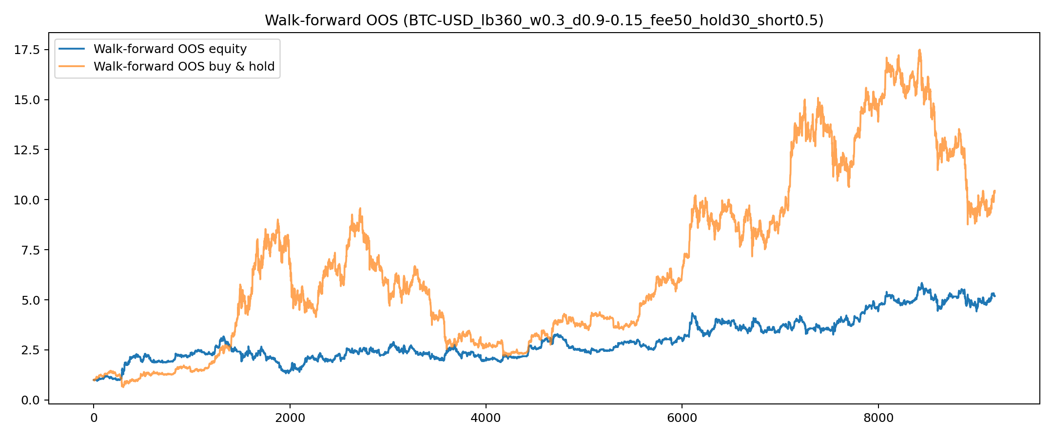
- fee10: ann_return 0.4376, Sharpe 0.9383, maxDD -0.5480
- fee25: ann_return 0.3716, Sharpe 0.7965, maxDD -0.5607
- fee50: ann_return 0.2615, Sharpe 0.5597, maxDD -0.5811
Takeaway: a viable 6h pocket appears to exist under fee stress. Turnover is higher than daily on this setup, which increases sensitivity to friction assumptions.
1h canon — stitched OOS
Canon: lb=2880, w=0.25, δ_hi/δ_lo=0.80/0.30, hold=720 bars, short_scale=0.5. BTC fee stress shown; ETH validated at fee=50 in this snapshot.
ETH (short0.5)
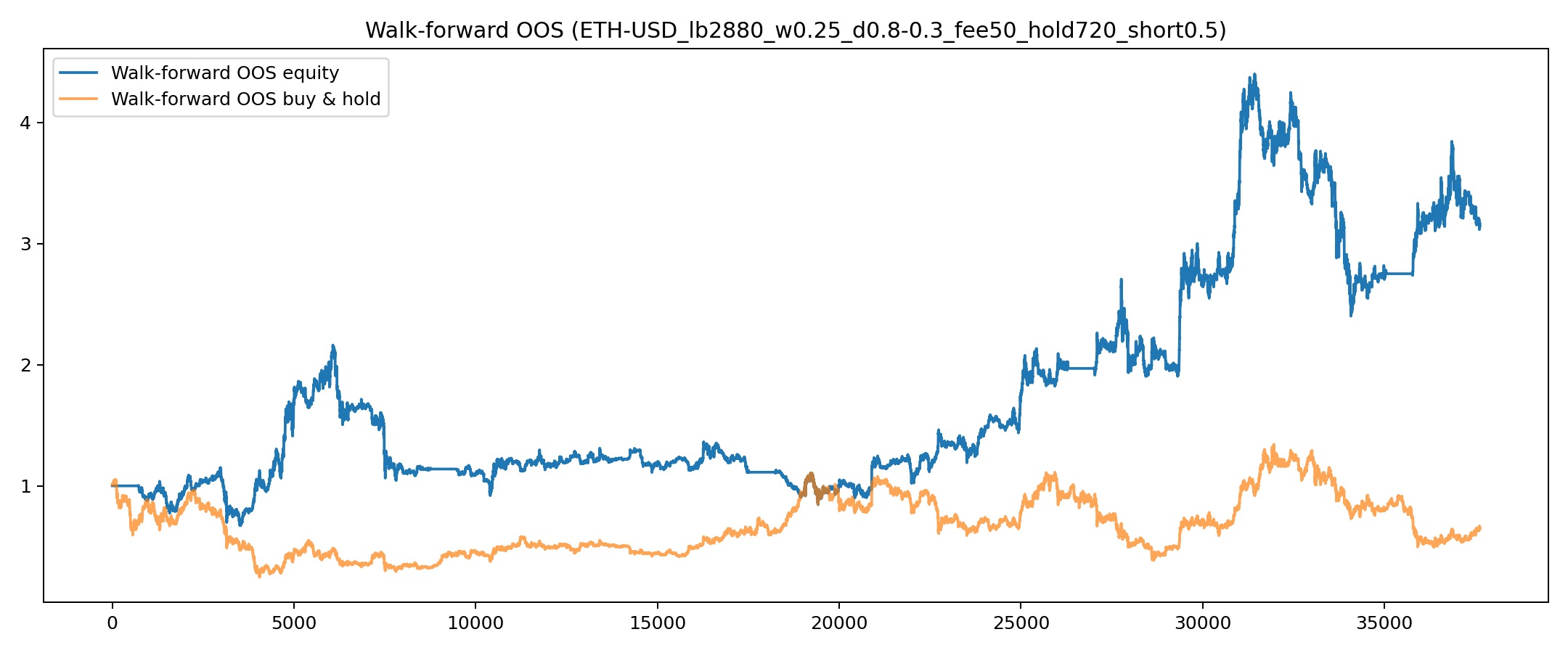
- fee10: ann_return 0.3156, Sharpe 0.6239, maxDD -0.5801
- fee25: ann_return 0.2977, Sharpe 0.5886, maxDD -0.5913
- fee50: ann_return 0.2681, Sharpe 0.5297, maxDD -0.6093
BTC (short0.5)
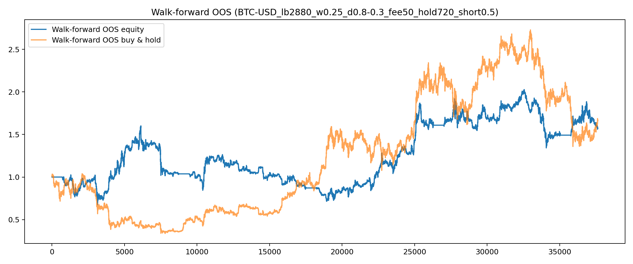
- fee10: ann_return 0.1533, Sharpe 0.3979, maxDD -0.5214
- fee25: ann_return 0.1355, Sharpe 0.3516, maxDD -0.5335
- fee50: ann_return 0.1058, Sharpe 0.2743, maxDD -0.5529
Takeaway: hourly remains viable in pockets but is more regime-sensitive. That sensitivity is expected intraday and is one reason the workflow keeps walk-forward and fee buckets as first-class tests.
10. Reproducibility and audit trail
Every run writes a bundle of artifacts (CSV/PNG/JSON). Meta files record:
- data source path and symbol
- full configuration snapshot
- bars-per-year constant
- window boundaries used for walk-forward
- summary metrics and output filenames
The objective is that any result can be reproduced from a config + data file without manual reconstruction.
11. Controller benchmark findings (1d)
A small controller benchmark was run on daily BTC and ETH using the same walk-forward stitched OOS protocol, the same fee buckets (10/25/50 bps), and the same long/short policy semantics. The comparison set included the progress-state gate, a Schmitt trigger hysteresis controller, a simple one-sided hysteresis controller, and a rolling sine/cosine phase-fit baseline (“sinefit”).
BTC-USD (1d)
- The progress-state gate remained the best controller in this benchmark at fee10 and fee25 with score 0.3695 / 0.3256, ann_return 0.1805 / 0.1641, Sharpe 0.4739 / 0.4304, maxDD -0.2984 / -0.2995, and 47 turns.
- At fee50, a more conservative Schmitt trigger could outperform the gate by reducing turnover materially. The strongest Schmitt pocket tested here was enter_z=0.8, exit_z=0.3, with score 0.2959, ann_return 0.0862, Sharpe 0.3691, maxDD -0.2092, and 10 turns.
- Interpretation: on BTC daily, the gate performs best under low/moderate friction, while a stricter hysteresis controller can become preferable once friction is high enough that turnover dominates.
ETH-USD (1d)
- The rolling sine/cosine phase-fit baseline showed a clear and localized dominance pocket at window=180, period=60. In that pocket it won all fee buckets: fee10 score 1.1277, ann_return 0.4661, Sharpe 1.2453, maxDD -0.3358, turns 16; fee25 score 1.1123, ann_return 0.4605, Sharpe 1.2302, maxDD -0.3368, turns 16; fee50 score 1.0865, ann_return 0.4511, Sharpe 1.2050, maxDD -0.3385, turns 16.
- Secondary sinefit wins appeared at window=180, period=90 and window=210, period=50, but these were materially weaker than the 180/60 pocket.
- Outside those narrow phase-fit pockets, the progress-state gate remained the best controller in the tested set. Interpretation: ETH daily appears to support a localized phase-style pocket, whereas the gate is the more stable default once that pocket is missed.
Takeaway: the controller benchmark does not support a single universal winner. Instead it suggests a more nuanced result: the progress-state gate is a strong default controller, especially on BTC and under low/moderate friction, while alternative stateful controllers can dominate in specific pockets (Schmitt under heavy BTC friction; sinefit in a narrow ETH daily phase pocket).
12. Limitations
- Friction is bucketed (bps per turn) rather than a full order-book model.
- Signal mapping is intentionally minimal; alternative features may change behaviour materially.
- Walk-forward uses calendar boundaries; alternative splits may produce different stress patterns.
- Crypto regime structure shifts; pockets can degrade over time.
13. Next methodological extensions
- Baseline comparisons (e.g. MA/trend) under identical windows and friction buckets
- Simple slippage models (extra bps per trade, volatility-scaled friction)
- Portfolio-level gating (multiple assets, shared risk budget)
- Config registry (public canon + optional private pockets)
Closing note
The main claim supported by this workflow is modest: a small deterministic gate can provide a reusable controller primitive with hysteresis and memory, and robust evaluation can be made cheap enough to run routinely.
Further Reading

Code and Reproducibility
The analysis pipeline used in this study is implemented in Python. All code used to generate the figures and statistical results presented in this work is available as open-source software:
github.com/hasjack/OnGravity/tree/main/python/bell-toy
This repository includes the full analysis pipeline, data ingestion routines, model fitting procedures, and scripts used to generate the figures presented in this paper.
Please consider funding this research on Research Hub

Content on this site is licensed under a Creative Commons Attribution 4.0 International License