Progress-State Bell Toy in Natural Mathematics

Jack Pickett - 12th April 2026

Progress-State Bell Toy

A Bell-style toy model is constructed from a primitive state built from sector and progress,

where $\sigma \in \{+1,-1\}$ denotes the current orientation sector and $p \in [0,1)$ denotes progress through that sector. The construction treats binary state and state progress as the fundamental variables. The sector label $\sigma$ supplies the observable state, while $p$ tracks advance toward the next flip.

An earlier exploratory draft introduces the orientation-based language of Natural Mathematics in heuristic form. The present note does not rely on the full axiomatic programme. It isolates one minimal sector-progress structure inspired by that draft and studies its consequences as a local Bell-style toy model.

Update Rule

Given a progress increment $\delta \ge 0$, the state is updated through

with total progress

flip count

and remainder

The updated sector is

The updated state is therefore $(\sigma',r)$. Progress accumulates continuously within a sector, and each boundary crossing flips the sector while preserving the remainder. When several boundaries are crossed in one update, only the parity of the number of crossings determines the final sector.

Example Updates

The update rule behaves as expected in simple test cases:

These examples confirm the intended behaviour: persistence within a sector, flipping on overflow, and retention of the remainder after the flip.

Binary Measurement Rule

The toy uses the simplest binary observable,

so the sector itself supplies the readout.

Bell Construction

A shared source emits pairs with common hidden variables: an initial sector $\sigma_0$, an initial progress $p_0$, and a shared latent parameter $\lambda$. Each wing then evolves locally according to its own setting.

The hidden-variable space is taken to be

with $\sigma_0$ sampled uniformly from $\{\pm1\}$, $p_0 \sim \mathrm{Unif}[0,1)$, and $\lambda \sim \mathrm{Unif}[-\pi,\pi)$. These source variables are taken to be statistically independent of the measurement settings.

For settings $a,a'$ on one wing and $b,b'$ on the other, local progress increments are defined by

Each wing updates independently, and the resulting outcomes are correlated in the usual CHSH form.

The correlations are computed as

and the CHSH combination is

Local Response Rule

A piecewise local response rule is introduced. Let

where $\mathrm{wrap}$ returns angular separation on $[-\pi,\pi)$. The local progress increment is taken to be

The parameter $w$ therefore sets the width of the local response window. Local alignment produces strong progress, while non-alignment produces weak progress.

Analytic Correlation Lemma

Because both wings share the same hidden source state, the product of the two binary outcomes depends only on the parity mismatch between the two local overflow counts. Writing

one can make the mechanism completely explicit.

Lemma

Assume $p_0 \sim \mathrm{Unif}[0,1)$ and $\delta(x,\lambda),\delta(y,\lambda) \in [0,1)$. Then

Proof

For fixed $\lambda$, each floor term $\lfloor p_0 + \delta(\cdot,\lambda)\rfloor$ is either $0$ or $1$. A parity mismatch occurs exactly when one of the two quantities crosses the overflow threshold and the other does not. Since $p_0$ is uniform on $[0,1)$, the set of mismatch values has measure $|\delta(x,\lambda)-\delta(y,\lambda)|$. Therefore the product $A_x B_y$ equals $-1$ on a set of that measure and $+1$ elsewhere, giving the stated conditional expectation.

Averaging over the shared hidden variable $\lambda$ yields

This expression shows that the Bell-type structure is controlled by the average mismatch in local progress increments under the shared hidden variable $\lambda$.

For the specific two-level rule used here, $\delta \in \{0.85,0.20\}$, so

and therefore

The correlations are thus determined by the extent to which the two local response windows disagree as functions of $\lambda$.

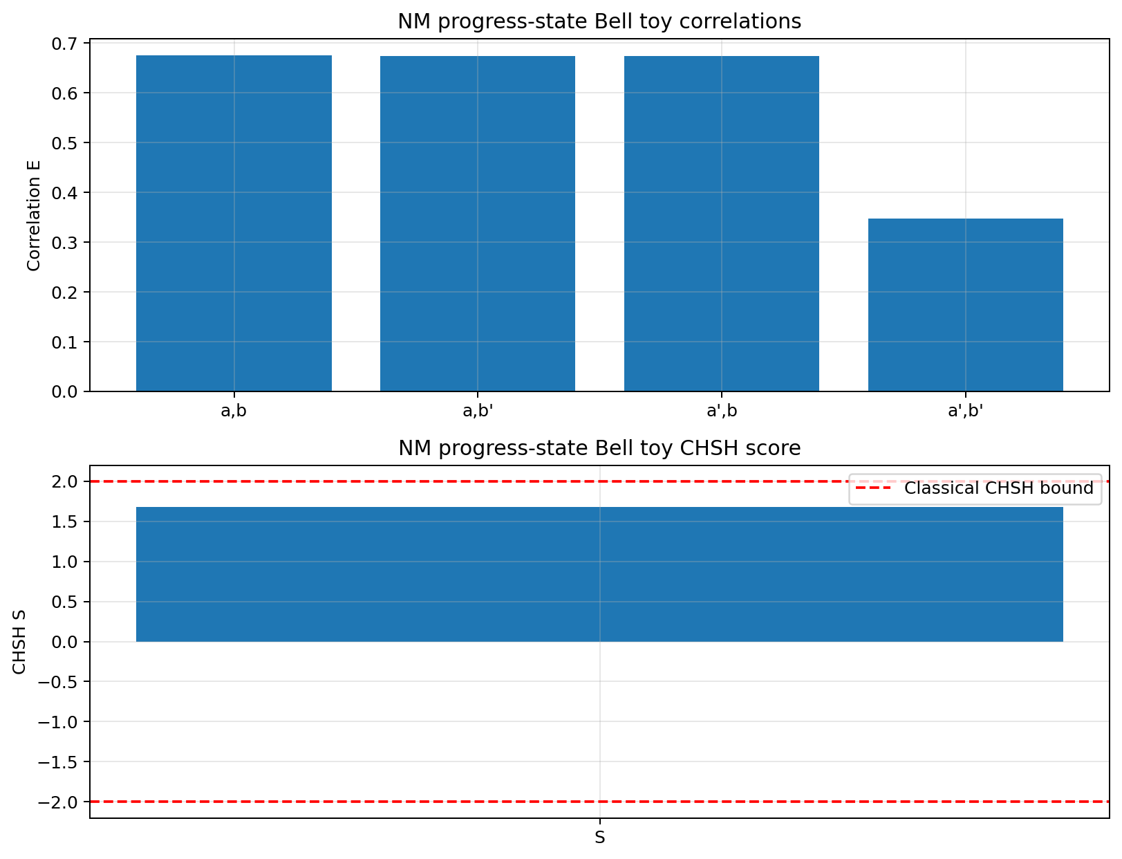
Figure 1: Representative progress-state Bell toy result for a fixed local response window. Top: the four Bell-setting correlations. Bottom: the corresponding CHSH score. Numerical values shown here and below are estimated by Monte Carlo sampling of $\Omega$ under the stated uniform source distribution.

Classicality

For each hidden state $\omega \in \Omega$, the toy assigns deterministic local binary outcomes $A_x(\omega), B_y(\omega) \in \{\pm 1\}$. The construction therefore lies within the standard local hidden-variable class, and the CHSH bound

follows by the usual theorem. The numerical sweep therefore illustrates how the response-window parameter moves the toy within the classical region.

Width Sweep

To test robustness, the response width is swept across four values:

• $\pi/6$
• $\pi/5$
• $\pi/4$
• $\pi/3$

The corresponding CHSH scores are

The CHSH score rises monotonically across the sweep. The response window therefore supplies a genuine control parameter for the toy.

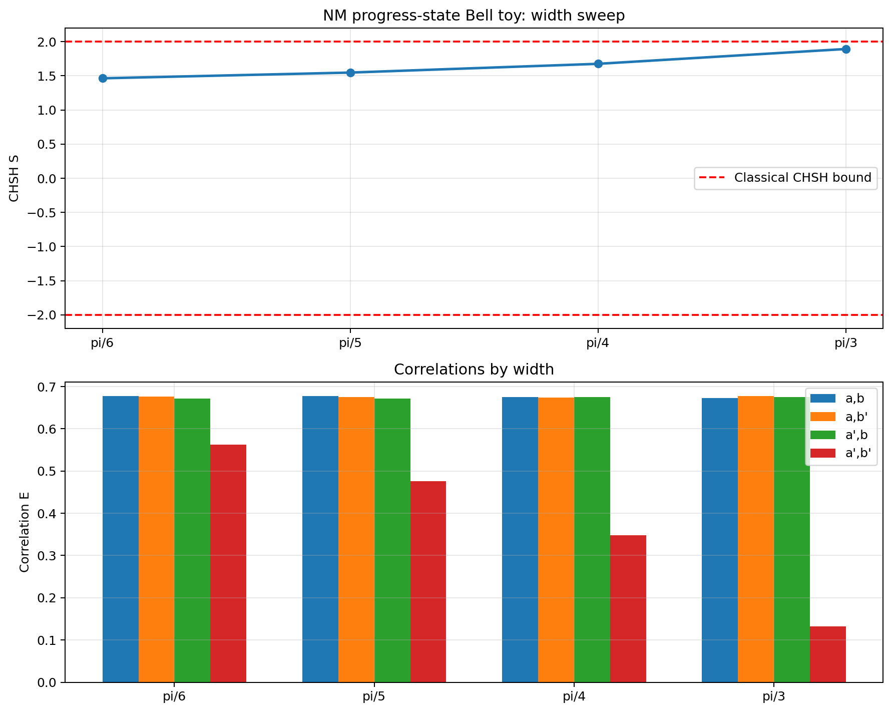
Figure 2: CHSH score as a function of response-window width $w$ for the progress-state Bell toy. Top: CHSH score across the width sweep. Bottom: the four setting-pair correlations across the same sweep. The score rises from $S \approx 1.46$at $w=\pi/6$ to $S \approx 1.89$ at $w=\pi/3$, approaching but not exceeding the classical bound.

Correlation Pattern

The increase in $S$ does not arise from all four correlations growing together. The three channels $E(a,b)$, $E(a,b')$, and $E(a',b)$ remain clustered near $0.67$ across the sweep. The main change occurs in the $E(a',b')$ channel, which falls steadily:

• $E(a',b') \approx 0.5627$ at $w=\pi/6$
• $E(a',b') \approx 0.4760$ at $w=\pi/5$
• $E(a',b') \approx 0.3482$ at $w=\pi/4$
• $E(a',b') \approx 0.1319$ at $w=\pi/3$

The rise in $S$ is therefore driven by one setting pair becoming progressively more exceptional than the other three. In the language of the analytic reduction above, this is the setting pair for which the two local response windows disagree most strongly as functions of $\lambda$.

Diagnostic Behaviour

Across the sweep, the mean progress increments and mean flip counts change only modestly. The dominant change appears in the same-sector agreement for the $a',b'$ channel. The width parameter therefore alters the pattern of sector agreement more strongly than the overall level of activity.

Interpretation

The progress-state Bell toy shows that a minimal sector-progress algebra, written in Natural Mathematics language as $(\sigma,p)$, supports a local Bell-style model with binary measurements and non-trivial setting-dependent correlations.

1. The $(\sigma,p)$ formalism supplies a working local update algebra with explicit binary readout.
2. The Bell-type structure depends strongly on the local response rule. The piecewise response preserves the sector structure clearly enough to produce a monotonic CHSH trend across the width sweep.
3. Widening the local response window drives the CHSH score upward toward the classical ceiling by suppressing one correlation channel while leaving the other three relatively stable.

The toy remains classical throughout the tested sweep. No Bell violation occurs. The result instead demonstrates that local sector-progress dynamics are sufficient to generate a structured and tunable Bell-type landscape.

Summary

The progress-state Bell toy provides a clean checkpoint for the toy phase. A primitive state space built from sector and progress, together with a flip-on-overflow update law, generates structured CHSH-style correlations under fully local rules. The score rises from approximately $1.46$ to $1.89$ as the local response window widens from $\pi/6$ to $\pi/3$, while remaining below the classical bound.